With data validation in Google Sheets, you can eliminate incorrect entries by checking the data as soon as you enter it. This allows you to confirm text, numbers, dates, and other types of data with simple rules you set up.
Because there are several types of validation rules you can apply to your dataset, let’s walk through each one individually so you can pick the one that fits best.
Validate Text
With the text validation feature in Google Sheets, you can check for entries that contain, don’t contain, or are the same as specific text. You can also validate the cell for an email address or URL.
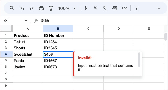
For example, we’ll validate the text in our cell to make sure it contains “ID” for our product numbers.
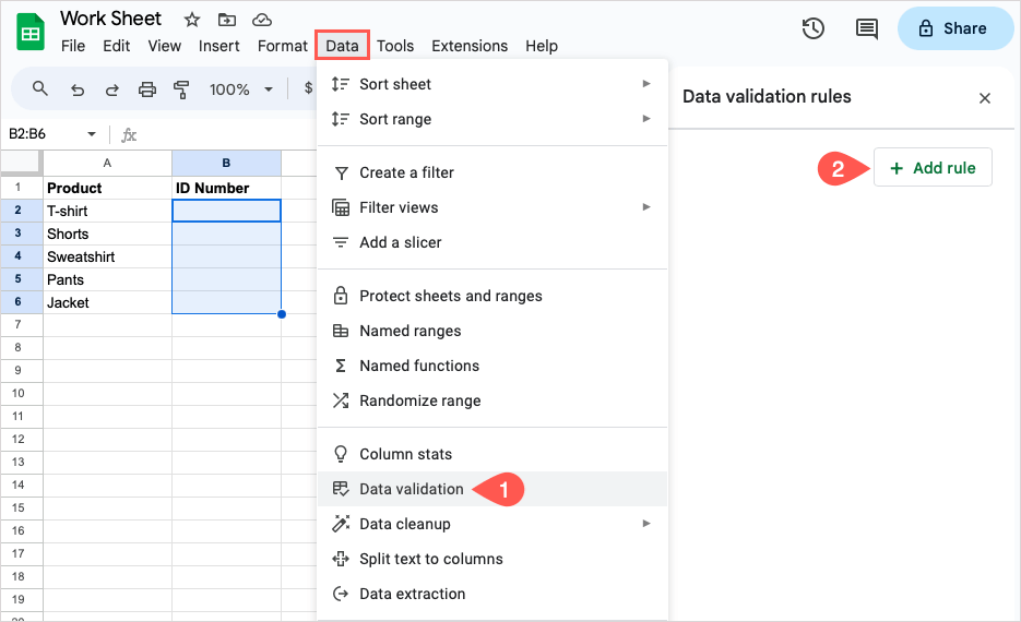
Select the cell or range and use Data > Data validation to open the sidebar and pick Add rule.
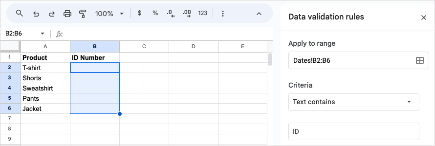
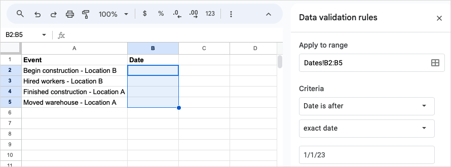
Apply to range: Confirm the cell or range and use the icon on the right to add another cell range. Note: As shown below, you should use the sheet (tab) name with the cell reference or data range. Our sheet name is Dates.
Criteria: Pick the text option you want to use and enter the text in the field beneath. For our example, we choose “Text contains” and enter “ID.”
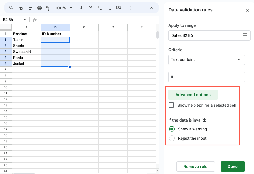
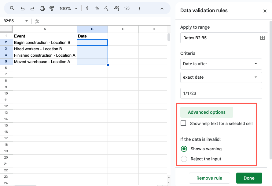
Advanced options: To show and enter help text or choose a warning or rejection for invalid data, expand Advanced options, and mark the ones you want to use.
Select Done to apply the rule. You can then test your data validation rule. Input a valid entry and then an invalid entry to make sure the rule works as you expect.
Validate Dates
For validating dates in Google Sheets, you have several options. You can check for a date on, after, before, or between as well as a valid date.
As an example, you may want to confirm that the dates entered fall after a particular date, such as January 1, 2023, for your company’s 2023 financials.
Select the cell or range and use Data > Data validation to open the sidebar and pick Add rule.
Apply to range: Confirm the cell or range and optionally add another.
Criteria: Pick the date option you want to use the drop-down menu or text field to pick or enter the corresponding date. For our example, we pick “Date is after,” choose “exact date,” and enter “1/1/23” in the field beneath.
Advanced options: Like the text validation above, you can expand this section to add help text and pick an invalid input action.
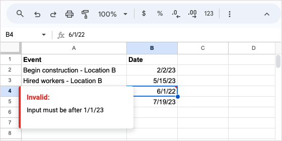
Select Done when you finish. You can then test your date validation by entering a valid and invalid date per your rule.
Validate Numbers
If you want to validate numbers in Sheets, you can set up a rule that checks for those greater than, less than, equal to, between, and more.
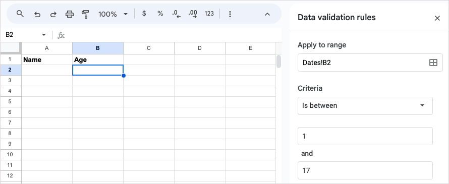
For this example, we want to confirm that the number entered is between 1 and 17 for parents entering their minor child’s age.
Select the cell or range, pick Data > Data validation, and choose Add rule.
Apply to range: Confirm the cell or range and optionally add another.
Criteria: Pick the date option you want to use and enter the text in the field beneath. For our example, we pick “Is between” and enter “1” in the first field and “17” in the second.
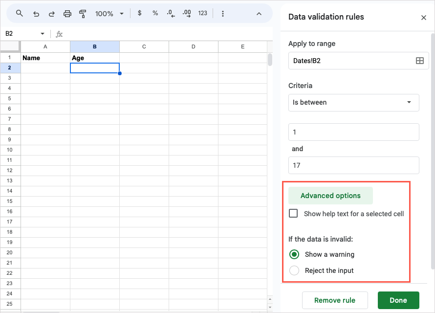
Advanced options: Like the above validations, expand this section to add help text and pick an invalid data action.
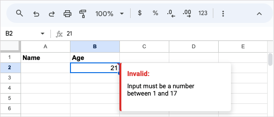
Select Done to apply the rule. Test your number validation rule by entering both a correct and incorrect number.
Create a Drop-Down List
Drop-down lists are another validation type you can use in Sheets. What’s different about these is that you can insert a drop-down list using the Insert or the Data menu. Either way, you’ll use the Data Validation sidebar to set up the list of items.
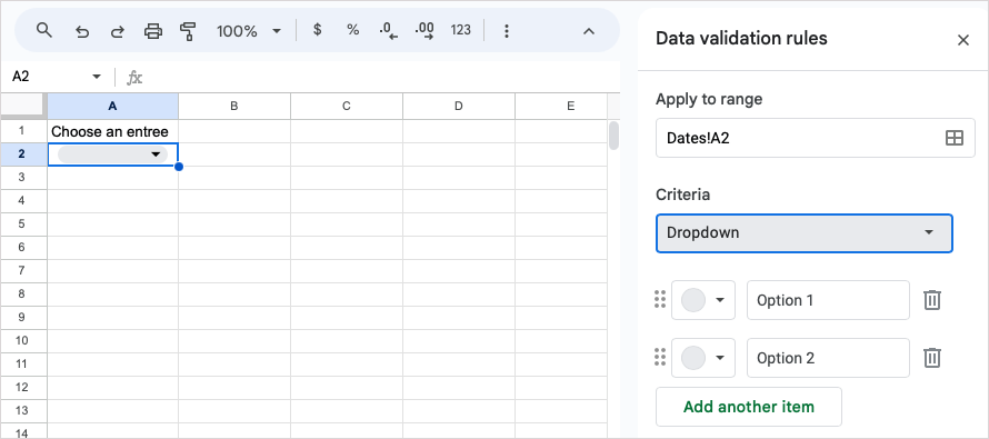
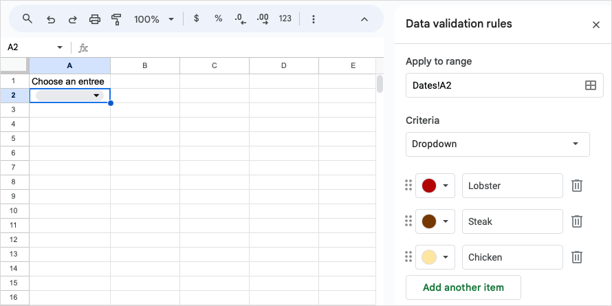
Here, we’ll set up a drop-down list to choose a menu item.
Do one of the following to add a drop-down list:
- Select the cell and pick Insert > Dropdown in the menu. The sidebar will open.
- Right-click the cell and pick Dropdown.
- Select the cell, pick Data > Data validation, and choose Dropdown in the Criteria menu in the sidebar.
Enter your list items in the Option 1 and Option 2 fields and use the Add another item button to include more. You can also reorder the items using the grid icons on the left of each.
Choose a color for each list item in the color palette drop-down box on the left.
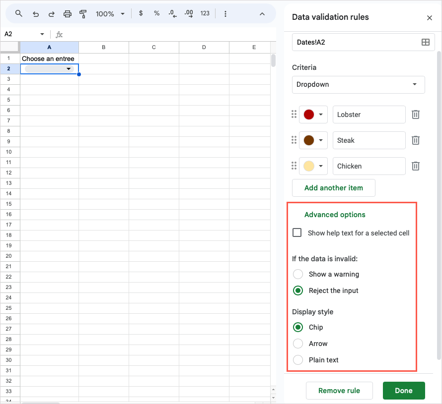
Advanced options: Expand this section to show help text, choose an invalid data action, and pick the display style for the list.
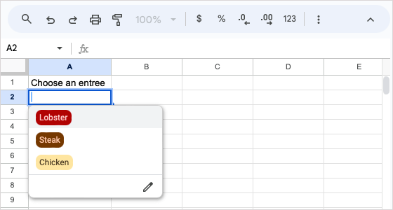
Select Done when you finish, and you’ll see your drop-down list ready to go.
Insert a Checkbox
Similar to the drop-down list validation above, you can add a checkbox to a cell using one of two options and customize the values in the Data Validation sidebar.
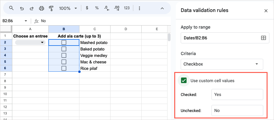
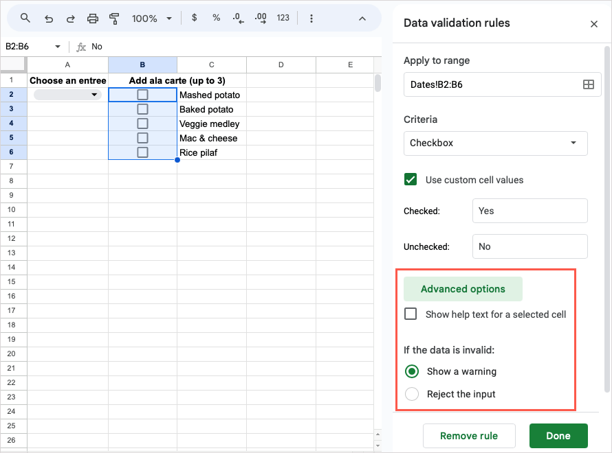
Here, we’ll add checkboxes to add dishes to our meals.
- Select the cell and pick Insert > Checkbox in the menu. The sidebar will open.
- Select the cell, pick Data > Data validation, and choose Checkbox in the Criteria menu in the sidebar.
To use specific values for the checked and unchecked box statuses, mark the option Use custom cell values and enter those you want to use. For our example, we enter “Yes” and “No.”
Advanced options: Expand this section to show help text and choose an invalid input action.
Select Done to apply the checkbox rule to the cell or range of cells.
Use a Custom Formula
One more way to use data validation is with a custom formula in Google Sheets. This is a good option when none of the above preset rules apply. You can do things like make sure the cell contains text or limit the number of characters in the cell.
As an example, we’ll set up the validation rule to check for text in the cell. If a number or date is entered, this invokes the invalid data action.
Select the cell or range and pick Data > Data validation.
Apply to range: Confirm the cell or range and optionally add another.
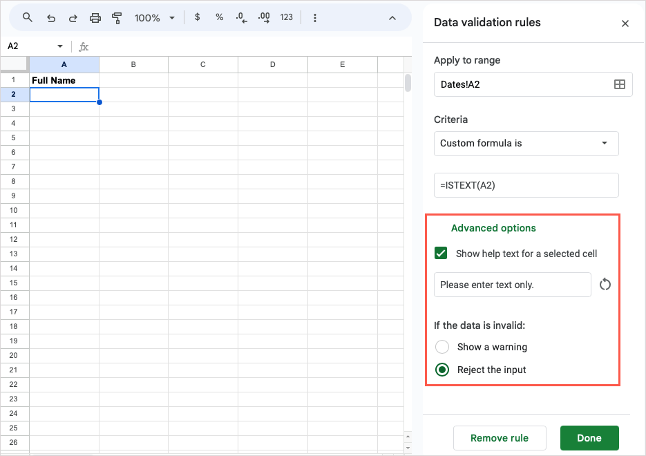
Criteria: Pick “Custom formula is” and enter the formula in the field beneath. Using our example, we enter the formula “=ISTEXT(A2)” to check that cell A2 contains text.
Advanced options: Expand this section to enter help text and choose an invalid data action. For our example, we’ll mark the option to show help text and enter a custom message to display along with rejecting the input.
Select Done to apply the rule. Then, give your new validation rule a test by entering both valid and invalid data to make sure the formula works as expected. In the screenshot below, you can see our message for an invalid entry.
Edit or Remove Data Validation
If after you set up a data validation rule, you want to change it or simply remove it, both are easy to do.
Select the cell or range containing the validation and choose Data > Data validation in the menu to open the sidebar.
Then, do one of the following:
- To edit a rule, select it, make your changes, and choose Done to save it.
- To remove a rule, hover your cursor over it and select the Delete (trash can) icon.
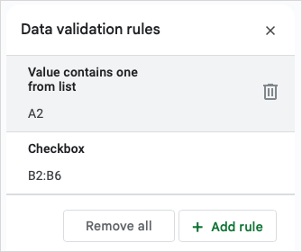
- To remove every rule in the list, use the Remove all button.
With the data validation feature in Google Sheets, you can make sure your data is entered correctly. Whether you pop up a warning message or provide drop-down list options, you can save yourself the aggravation of checking for invalid data later.
If you also use Microsoft applications, look at how to create a drop-down list in Excel too.

