How many of these will you use?
Whether you import data into Google Sheets or manually enter it, you can have situations where you need to change or correct text. Using the Google Sheets text functions on our list, you can save time by making several changes quickly and at once.
Convert a Number to Text: TEXT
Starting with a simple way to convert a number to text using a specified format is the TEXT function. You can use it for a date, time, percentage, currency, or similar number.
The syntax for the formula is TEXT(number, format), where you can use the exact number or a cell reference for the first argument. Depending on the format you want to use, you can visit the Google Docs Editors Help page for the list of over a dozen options for the second argument.
As an example, we’ll format the time 22:30 in a 12-hour format with AM or PM and as text using this formula:
=TEXT(“22:30”,”hh:mm AM/PM”)
For another example, we’ll format the number in cell A1 as text with a percent sign using this formula:
=TEXT(A1,”0%”)
Combine Text: CONCATENATE
If you want to join two strings of text, you can use the CONCATENATE function. You may have a first name and last name, city and state, or similar that you want to combine into a single cell.
The syntax is CONCATENATE(string1, string2,…), where you can use the text or cell references for the arguments.
In this example, we’ll combine the text in cells A1 through D1 into a single string with this formula:
=CONCATENATE(A1:D1)
If you want to place a space between the words, you can insert a blank space within quotation marks between each cell reference using this formula:
=CONCATENATE(A1,” “,B1,” “,C1,” “,D1)
For another example, we’ll combine the text “First name: ” with the text in cell A1 with this formula:
=CONCATENATE(“First name: “,A1)
Combine Text With a Delimiter: TEXTJOIN
The TEXTJOIN function is similar to CONCATENATE for combining text. The difference is that you can use a delimiter (separator) and combine arrays with TEXTJOIN.
The syntax is TEXTJOIN(delimiter, empty, text1, text2,…). For the delimiter argument, place the space, comma, or other delimiter in quotes and for the empty argument, use True to exclude empty cells or False to include them.
As an example, we’ll join the text in the cell range A1 through C2 with a space as the delimiter and TRUE to ignore the empty cell (A2). Here’s the formula:
=TEXTJOIN(” “,TRUE,A1:C2)
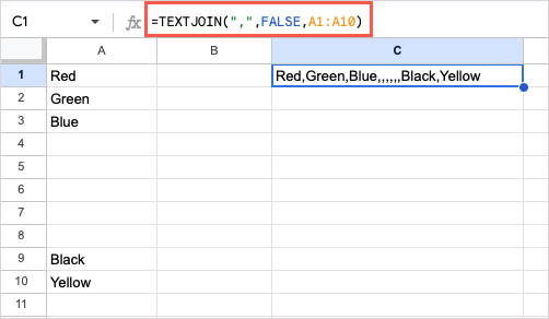
For another example, we’ll combine the text in cells A1 through A10 with a comma as the delimiter and FALSE to include the empty cells (A4 through A8) so you can see how the result looks. Here’s the formula:
=TEXTJOIN(“,”,FALSE,A1:A10)
Tip: If you want to combine numbers, you can use the JOIN function.
Separate Text: SPLIT
Maybe you want to do the opposite of the above and separate text rather than combine it. For this, you can use the SPLIT function.
The syntax is SPLIT(text, delimiter, split_by, empty). Use the split_by argument with True (default) to separate the text around each character in the delimiter, otherwise use False. Use the empty argument with True (default) to treat consecutive delimiters as one, otherwise use False.
Here, we’ll split the text in cell A1 using a space as the delimiter and the defaults for the other arguments with this formula:
=SPLIT(A1,” “)
For another example, we’ll split the text in cell A1 using “t” as the delimiter. This removes the “t” like it removes the space delimiter above and leaves the rest of the text. Here’s the formula:
=SPLIT(A1,”t”)
Now, if we add FALSE as the split_by argument, this formula separates the text only at the “t[space]” mark:
=SPLIT(A1,”t “,FALSE)
Compare Text: EXACT
Are you working on comparing data in your sheet? Using the EXACT function, you can compare two strings of text and receive a simple True or False result for whether they match or not.
The syntax is EXACT(text1, text2), where you can use text or cell references for the arguments.
As an example, we’ll compare the two text strings in cells A1 and B1 with this formula:
=EXACT(A1,B1)
For another example, we’ll compare the text in cell A1 with “Google” using this formula:
=EXACT(A1,”Google”)
Change Text: REPLACE and SUBSTITUTE
While you can use the Find and Replace feature in Google Sheets, you may need to be more specific than the feature allows. For instance, you might want to change a letter in a particular spot or only a certain instance of text in a string. In this case, you can use either REPLACE or SUBSTITUTE.
Although similar, each function works slightly differently, so you can use whichever meets your needs best.
The syntax for each is REPLACE(text, position, length, new) and SUBSTITUTE(text, search_for, replace_with, occurrence). Let’s walk through a couple of examples and how to use the arguments.
REPLACE
Here, we want to replace “William H Brown” with “Bill Brown,” so we’ll use the REPLACE function and this formula:
=REPLACE(A1,1,9,”Bill”)
To break down the formula, A1 is the cell with the text, 1 is the starting position to replace, 9 is the number of characters to replace, and Bill is the replacement text.
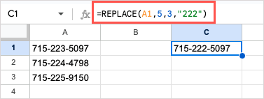
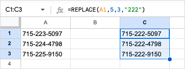
As another example, we have phone numbers stored as text and need to change the prefix for each. Since each prefix is different, we can use REPLACE to specify the position and number of characters for the replacement. Here’s the formula:
=REPLACE(A1,5,3,”222″)
Tip: To change multiple cells in a column, you can drag the formula down to apply it to the subsequent rows as shown below.
SUBSTITUTE
For an example of the SUBSTITUTE function, we want to replace “new york” with “New York” and will add the occurrence argument to make sure we only change the first instance in our string. Here’s the formula:
=SUBSTITUTE(A1,”new york”,”New York”,1)
To break down this formula, A1 contains the text, “new york” is the text we search for, “New York” is the replacement, and 1 is the first occurrence of the text.
If you were to remove the occurrence argument in the above formula, the function would change both instances to “New York” by default as you can see here:
=SUBSTITUTE(A1,”new york”,”New York”)
Change the Letter Case: PROPER, UPPER, and LOWER
If you import data from another source or mistype during data entry, you may end up with mismatched letter cases. Using the PROPER, UPPER, and LOWER functions, you can quickly correct it.
The syntax for each is simple as PROPER(text), UPPER(text), and LOWER(text) where you can use a cell reference or the text for the argument.
To capitalize the first letter of each word in a text string, you can use the PROPER function and this formula:
=PROPER(A1)
To change the letters to all uppercase, use the UPPER function and this formula:
=UPPER(A1)
To change the letters to all lower case, use the LOWER function and this formula:
=LOWER(A1)
Remember, you can also enter the exact text for all three functions within quotes as follows:
=PROPER(“online tech TIPS”)
Obtain Part of a Text String: LEFT, RIGHT, and MID
Maybe you need to extract part of a text string. You may have data mixed in with other data or want to use a portion of a string for something in particular. You can use the LEFT, RIGHT, and MID functions to get the part you need.
The syntax for each is LEFT(string, num_characters), RIGHT(string, num_characters), and MID(string, start, length). You can use a cell reference or the text as the string argument in each.
For an example of the LEFT function, we’ll extract the first three characters from the left using the text in cell A1 with this formula:
=LEFT(A1,3)
For an example of the RIGHT function, we’ll extract the first four characters from the right using the same cell with this formula:
=RIGHT(A1,4)
For an example of the MID function, we’ll extract the name “Jane” from the text in the same cell.
=MID(A1,6,4)
In this MID example, a 6 for the start argument selects the 6th character from the left. Remember that all characters count, including spaces and punctuation. Then, a 4 for the length argument selects four characters.
Get the Length of a Text String: LEN and LENB
When you plan to do something specific with your data, such as copy and paste or export it for use elsewhere, you might need to be cautious about the character count. With LEN, you can get the number of characters in a text string, and with LENB, you can get the count in bytes.
The syntax for each is LEN(string) and LENB(string), where again, you can use a cell reference or text as the argument.
Here, we’ll get the character count for the text in cell A1 with this formula:
=LEN(A1)
With this formula, we’ll get the character count for the text in cell A1 but as bytes instead:
=LENB(A1)
Remove Extra Spaces: TRIM
If you need to clean up your data from leading, trailing, or miscellaneous extra spaces, you can use the TRIM function.
The syntax is TRIM(text), where you can use a cell reference or text for the argument.
Here, we’ll remove the spaces from the text string in cell A1 with this formula:
=TRIM(A1)
Next, we’ll remove extra spaces from the specific text “ Online Tech Tips” with this formula:
=TRIM( “Online Tech Tips”)
Tackle Your Text With Google Sheets Functions
Google Sheets offers many features for working with text. You can wrap text, change the format, hyperlink it, and more. However, when you have a lengthy dataset, the Google Sheets text functions can help you tackle your text changes quicker and more efficiently. Will you give one or two a try?
For related tutorials, look at how to use Google Sheets formulas for arrays.


