Make sure your data goes pop
Highlighting a cell, text, or part of text in a cell is the best way to draw attention to your data in Google Sheets. You can highlight text to make a reminder or to organize your data in a more readable manner. But Google Sheets lacks the highlight tool available in Google Docs. So we’ll show you several different ways to do it. You can opt for manual highlighting by changing the cell’s background or text color. Or you can use Conditional Formatting to automatically highlight text containing specific words or phrases.
1. Highlight Cells
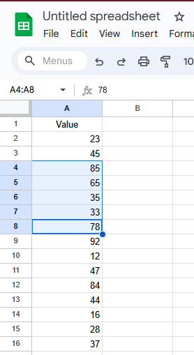
Highlighting the entire cell is pretty straightforward. You can choose to highlight only one or a group of cells. Follow these steps:
- Select the cell or a group of cells you want to highlight.
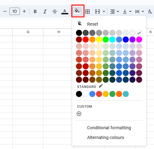
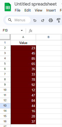
- Select the Fill color icon from the toolbar, and choose the highlight color you want.
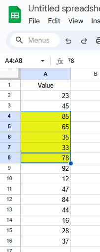
- The selected cells will automatically become highlighted with a different fill color than the others.
And that’s all there is to it. Highlighting cells might be the easiest thing to do in Google Sheets.
2. Highlight Text
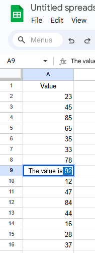
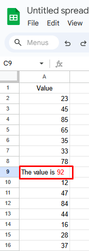
If you don’t want to highlight the whole cell but only the data inside it, you can do it by changing the text color. It doesn’t matter if it’s a particular value, the whole text, or just a part of the text in a cell you want to highlight; the concept is the same.
- Select the text within the cell or part of the text you want to highlight. Double-click the cell with your cursor to access the text to do this.
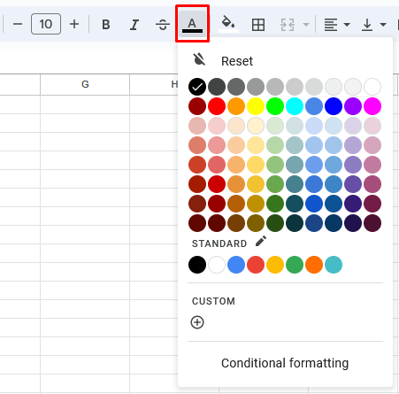
- Select the Text color icon from the main toolbar, and choose the desired color.
- The selected text will automatically change to the color you chose from the color palette.
Note: You can use as many colors as you want to highlight your text. But remember that some colors might be difficult to read depending on the cell background color. You can combine cell and text highlight methods to achieve different effects. You can also change the formatting style of your text to Bold, Italic, or Strikethrough to put even more emphasis on the text or a cell.
3. Conditional Formatting
For data analysis, you can format the cells based on their content. For example, you can change the background color of cells with the same value. Conditional formatting will save you time if you need to highlight several different cells with the same value and you don’t want to manually search for them to select and highlight those values.
Let’s see how to automatically highlight cells that begin, end, or contain a specific value, word, or phrase, changing only the conditional formatting rules.
Note: Conditional formatting is less powerful in Google Sheets compared to Microsoft Excel. The former limits you to 50 rules per sheet, while you can create up to 256 rules in Excel to highlight your data.
1. Highlight Text That Begins With a Specific Word
- Select a cell (or multiple cells) that contains a specific word, phrase, or value.
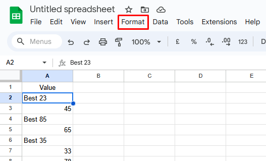
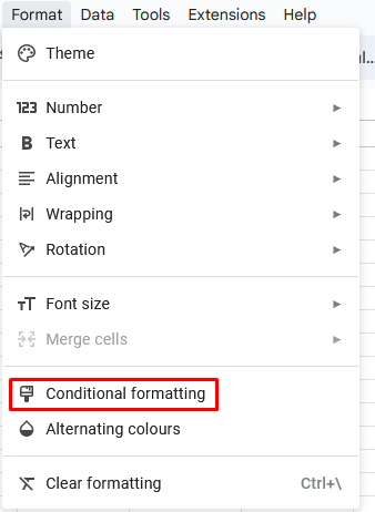
- Open the Format menu from the ribbon at the top of the screen.
- Select Conditional Formatting from the drop-down menu. The Conditional Formatting menu will open on the right side of the Google Sheet.
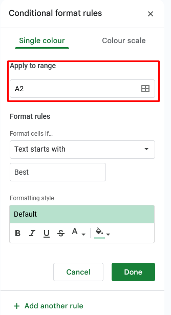
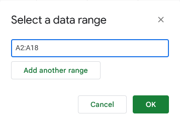
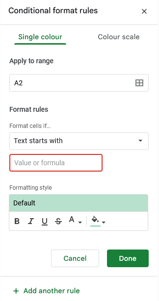
- If you want to apply Conditional Formatting to multiple cells that contain the same word, you’ll have to input the range to which the formatting will be applied. Click on the Apply to Range box.
- When the dialog box opens, type in the range of cells where you want to apply the formatting. Look at the cell numbers and column letters and type in the range— e.g. A2:A16. This will highlight the cells that meet the conditional formatting rule .
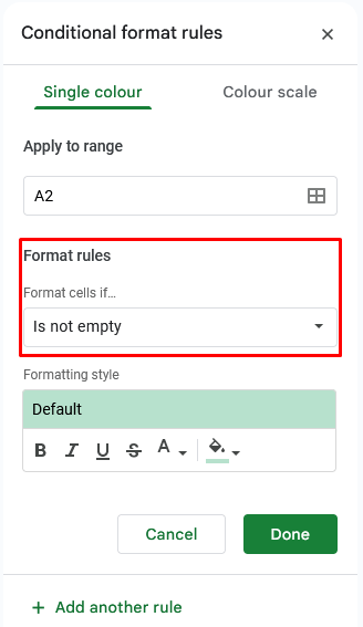
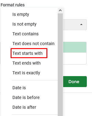
- In the Conditional Formatting menu, under Format Rules (or Conditional format rules), click on the drop-down menu for Format cells if…
- Select Text starts with from the drop-down menu.
- In the Value or formula box, type in the specific word (or a custom formula) with which the cell begins.
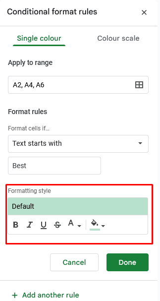
- In the Formatting Style section, you can select the text and background color you want added to the text or the whole cell and text formatting options such as Bold, Italic, and Strikethrough.
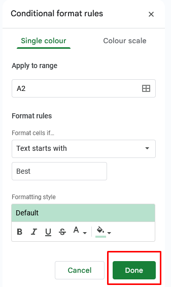
- When you select all the desired options in Formatting Style, hit the Done button.
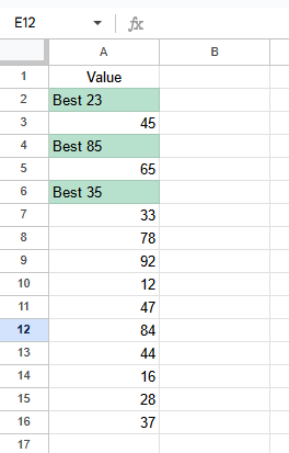
The cells containing a specific word will be highlighted automatically (in our example”, the word is “Best”).
2. Highlight Text That Ends With a Specific Word
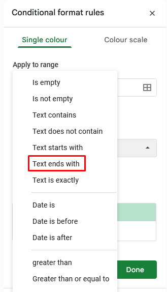
You can also highlight all the cells that end with a specific word. The steps are almost the same. However, when you come to the point where you need to select Format rules, You’ll choose Text ends with from the drop-down menu.
All the steps before and after this are the same as described in the previous section. Once you are ready to apply the highlight to all the cells that end with a specific word, phrase, or value, hit the Done button.
3. Highlight Text That Contains a Specific Word
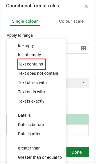
You probably guessed that to highlight text that contains a specific word you have to follow the same steps as previously described in the Conditional Formatting section. But when you reach the point to select Format rules, you’ll choose Text contains from the drop-down menu.
Select the formatting styles you desire and hit the Done button to finish.
Manually highlighting text gives you precise control over the selection process, allowing you to emphasize specific data points, labels, or insights. This hands-on method is ideal for smaller datasets.
On the other hand, automatic highlighting with conditional formatting offers efficiency and scalability. It allows you to set up rules that dynamically highlight cells based on specific criteria, making it perfect for larger datasets. After using conditional formatting, you can also filter your spreadsheet data by color.
Whether you choose the manual or automatic route, highlighting the correct text enhances the clarity and readability of your spreadsheets, so keep experimenting with both methods.

