There are 5 good reasons why you want to do this
If you are used to using older versions of Excel, the conditional formatting options in Excel 2007, 2010, and 2013 will amaze you. So why would you want to bother using conditional formatting? Well, here are a couple of reasons why I love using this feature of Excel:
1. To make your data more visually appealing.
Table of Contents
2. To make your spreadsheets easier to understand at a glance.
3. To identify certain types of numbers for help in problem solving.
4. To assist you in drawing conclusions from your data.
5. To visually display to the user what is “good” or “bad” by using green and red.
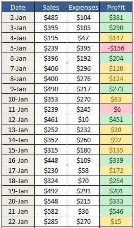
Now, you can use conditional formatting to format every cell in a range based on your own criteria (and there are a lot of formatting options to choose from). For example, if you have a profit sheet and you want to color code all profits greater than $200 as green and all profits less than $200 as yellow and all losses as red, then you can use conditional formatting to quickly do all the work for you.
Conditional Formatting in Excel
Conditional formatting enables you to format significant amounts of data quickly and easily – while still being able to distinguish different types of data. You can create rules for the formatting options that will allow Microsoft Excel to auto-format for you. You really only have to follow three simple steps.
Step 1: Select the cells you want to format.
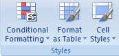
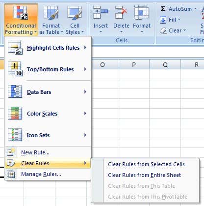
Step 2: Click the Conditional Formatting button under the Home menu, Styles section.
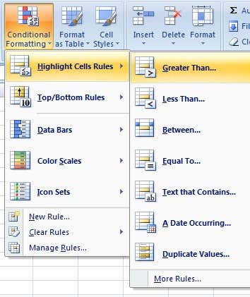
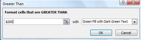
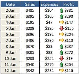
Step 3: Select your rules. There are Highlight Cells Rules and Top/Bottom Rules at the top that let you do comparisons with values. For this example, we imposed three rules. The first was that any value greater than $200 was green.
It’s worth noting that only the Highlight Cells Rules section can also be used to compare a dataset to another dataset. Everything else will just use the one dataset that you have highlighted and compare the values against each other. For example, when using the Greater Than rule, I can compare values from A1 to A20 against a specific number or I can compare A1 to A20 against B1 to B20.
The same logic was applied to the second and third rules. The second rule was that anything between $0 and $200 was formatted yellow. The third rule was that anything less than $0 was formatted red. Here is what a portion of the finished spreadsheet looks like.
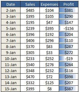
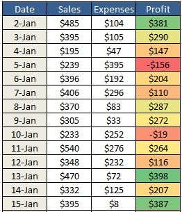
If you do not like these formatting options, Excel has many different new Conditional Formatting options that you can use from. For example, you can insert icons like colored arrows (Icon Sets), bar charts like in the second example (Data Bars), or even a range of automatically selected colors like in the last example (Color Scales). These three options only compare values from the same dataset. If you select A1 to A20, it’ll only compare those values against each other.
If you later decide that you don’t want your cells to be conditionally formatted, all you have to do is clear the formatting. To do this, select the Conditional Formatting button and select Clear Rules. Then, select whether you want to clear the rules from only the selected cells or from the entire worksheet.
Also, if you have created several rules, you might forget what rules you have applied to what cells. Since you can apply many rules to the same set of cells, it can become quite confusing especially if someone else created the spreadsheet. To see all the rules, click on the Conditional Formatting button and then click on Manage Rules.

When you have more than one rule applied to the same range of cells, the rules are evaluated in order from higher precedence to lower precedence. By default, the newest rule added will have the higher precedence. You can change that by clicking on the rule and then using the up and down arrow buttons to change the order. Also, you can click the dropdown at the very top and see the rules for only the current selection or for each sheet in the workbook.
There is also a checkbox called Stop If True, which I won’t go into detail here because it’s quite complicated. However, you can read this post from Microsoft that explain it in great detail.
New Conditional Formatting Options Excel 2010
Just about everything is the same in Excel 2010 when it comes to Conditional Formatting that was included in Excel 2007. However, there is one new feature that really makes it much more powerful.
Earlier I had mentioned that the Highlight Cells Rules section lets you compare one set of data to another set of data on the same spreadsheet. In 2010, you can now reference another worksheet in the same workbook. If you try to do this in Excel 2007, it will let you select the data from another worksheet, but will give you an error message when you try to click OK at the end.
In Excel 2010, you can now do this, but it’s a bit tricky so I’m going to explain it step by step. Let’s say I have two worksheets and on each sheet I have data from B2 to B12 for something like profit. If I want to see which values in B2 to B12 from sheet 1 are greater than the B2 to B12 values of sheet 2, I would first select the B2 to B12 values in sheet 1 and then click on Great Than under Highlight Cells Rules.

Now click on the cell reference button that I have shown above. The box will change and the cursor icon will become a white cross. Now go ahead and click on sheet 2 and select ONLY cell B2. Do NOT select the entire range of B2 to B12.

You’ll see that the box now has a value of =Sheet2!$B$2. We’re going to need to change this to =Sheet2!$B2. Basically, just get rid of the $ that comes before the 2. This will keep the column fixed, but allow the row number to change automatically. For whatever reason, it won’t just let you select the entire range.
Click the cell reference button again and then click OK. Now the values in sheet 1 that are greater than sheet 2 will be formatted according to the formatting options you chose.

Hopefully, that all makes sense! When looking at Excel 2013, there doesn’t seem to be any new features when it comes to conditional formatting. As a last tip, if you feel that the default rules don’t match what you are trying to accomplish, you can click the New Rule option and start from scratch. What’s great about creating a new rule is that you can use a formula to determine which cells to format, which is very powerful.

Even though conditional formatting looks relatively easy and simple on the surface, it can become quite complex depending on your data and your needs. If you have any questions, feel free to post a comment. Enjoy!