How to Filter in Google Sheets

When you’re working with large datasets, it’s useful to know how to filter in Google Sheets.

There are two ways to do this. You can use filter views in the Google Sheets menu, which lets you customize specific ways to filter the data in the sheet that you can reuse. A more dynamic method to filter data in Google Sheets is using the FILTER function.

In this article, you’ll learn how to use both methods.

Create a Filter View in Google Sheets

In this method, you’ll learn how to apply a filter that will show you only data from a large dataset that you want to see. This filter view will hide all other data. You can also combine filter parameters for more advanced filter views as well.

How to Create a Filter View

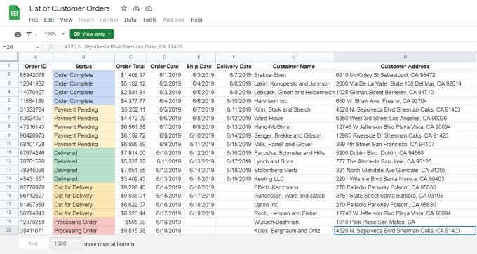
As an example, imagine you have a set of data that includes product purchases made by customers. The data includes names, addresses, emails, phone numbers, and more.

For this example, let’s say you want to see only customers from Playa Vista, CA, and only customers who have a “.gov” email address.

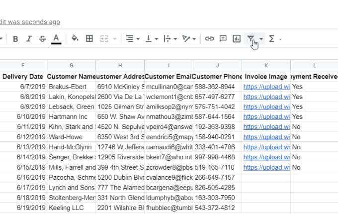
1. To create this filter, select the Create a Filter icon in the menu. This icon looks like a funnel.

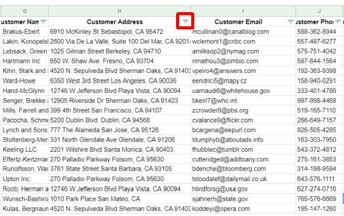
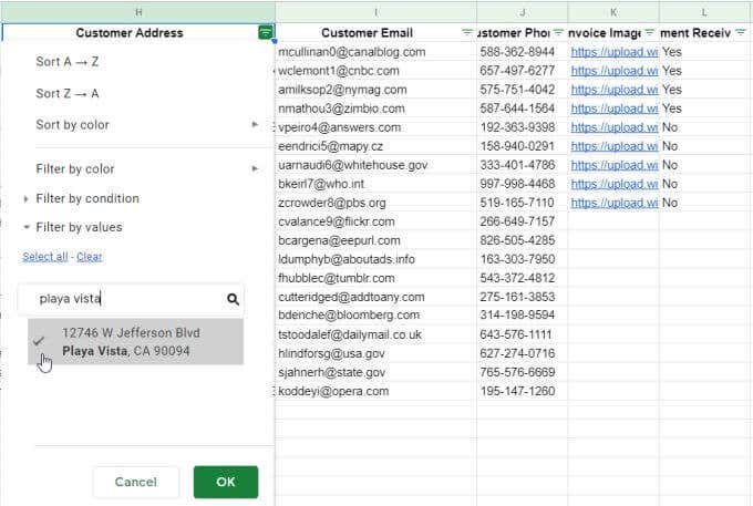
2. You’ll see small filter icons appear on the right side of each column header. Select this funnel icon at the top of the Customer Address field to customize the filter for this field.

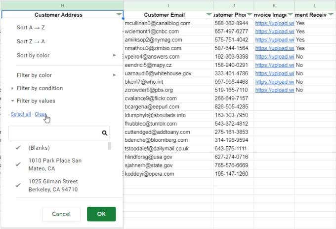
3. This will open a window where you can customize the filter options. Select the arrow to the left of Filter by values. Select Clear to deselect all entries in that field.

Note: This is an important step because it resets the view from showing all records to showing none. This prepares Excel to apply the filter you’re going to create in the next steps.

4. Type the text in the field below that you want to filter the field by. In this example, we’ll use “Playa Vista” and select the search icon to see only those records that contain that text. Select all of the records that show up in the results list. This customizes your filter so that only the items you select will be displayed in the spreadsheet.

4. Once you select the OK button, you’ll see the data in your sheet filtered so that only customers from Playa Vista are displayed.

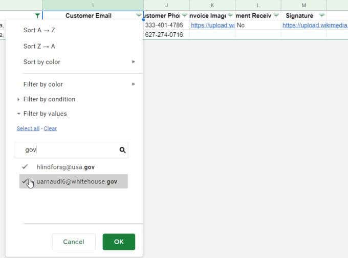
5. To filter on a second field, select the filter icon at the top of that field. Repeat the process above to create the filter. Clear all entries, type the “gov” text to filter out any email addresses that don’t contain “gov,” select those entries, and select OK.

Now you’ve customized your filter so that only the records in the dataset you care about are displayed. So that you don’t have to repeat this process every time you open the spreadsheet, it’s time to save the filter.

Saving and Viewing Filter Views

When you’re done setting up your filter, you can save it as a filter view that you can enable at any time.

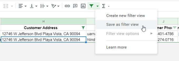
To save a filter view, just select the dropdown arrow next to the filter icon and select Save as filter view.

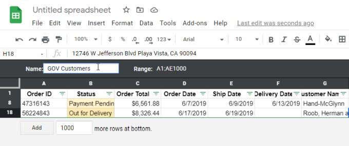
You’ll see a dark gray field open at the top of the spreadsheet. This will show you the selected range that the filter applies to and the name of the field. Just select the field next to Name and type the name you’d like to apply to that filter.

Just type the name and press Enter.

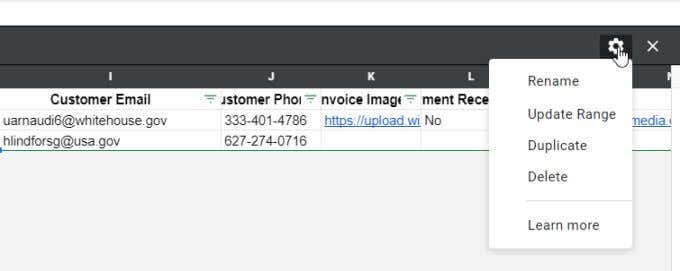
You’ll notice on the right side of the gray bar that there’s a gear icon. Select this icon to see filter options.

Available options include:

• Rename the filter
• Update the range that the filter applies to
• Duplicate the filter to update it without affecting the original filter
• Delete the filter

You can turn off the filter you’ve enabled at any point simply by selecting the filter icon again.

Note that when any filter is enabled, the filter icon will turn green. When you disable the filters, this icon will turn back to black. This is a quick way to see the entire dataset or if any filter has removed data from the current view.

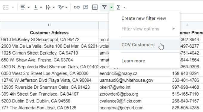
Later, if you want to re-enable any of the filters you’ve created, just select the dropdown arrow next to the filter icon. You’ll see the filters you’ve saved appear in the menu. Just select that filter to enable it whenever you like.

This will filter the view again using the filter settings you’ve configured.

Using the FILTER Function

Another option to filter in Google Sheets is using the FILTER function.

The FILTER function lets you filter a dataset based on any number of conditions you choose.

Let’s take a look at using the FILTER function using the same Customer Purchases example as the last section.

The syntax of the FILTER function is as follows:

FILTER(range, condition1, [condition2, …])

Only the range and one condition for filtering are required. You can add as many additional conditions as you like, but they aren’t required.

The parameters of the FILTER function are as follows:

• range: The range of cells you want to filter
• condition1: The column or rows that you want to use to filter results 
• conditionX: Other columns or rows you’d also like to use to filter results

Keep in mind that the range you use for your conditions needs to have the same number of rows as the entire range.

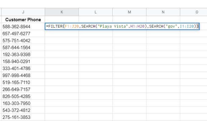
For example, if you want to create the same filter as the first part of this article, you’d use the following FILTER function.

=FILTER(F1:J20,SEARCH(“Playa Vista”,H1:H20),SEARCH(“gov”,I1:I20))

This grabs the rows and columns from the original table of data (F1:J20) and then uses an embedded SEARCH function to search the address and email columns for the text segments that we’re interested in.

The SEARCH function is only needed if you want to look for a text segment. If you’re more interested in an exact match, you can just use this as the condition statement instead:

I1:I20=”nmathou3@zimbio.com”

You can also use other conditional operators, like > or < if you want to filter values greater than or less than a fixed limit.

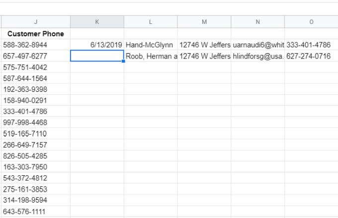
Once you press Enter, you’ll see the results of the FILTER function as a results table.

As you can see, only the columns in the range you selected in the first parameter of the function are returned. So it’s important to place the FILTER function in a cell where there’s room (enough columns) for all of the results to appear.

Using Filters in Google Sheets

Filters in Google Sheets are a very powerful way to dig through very large sets of data in Google Sheets. The FILTER function gives you the flexibility of keeping the original dataset in place but outputting the results elsewhere.

The built-in filter feature in Google Sheets lets you modify the active dataset view in whatever way you’re interested at any given moment. You can save, activate, deactivate, or delete filters however you like.

Do you have any interesting tips to offer for using filters in Google Sheets? Share those in the comments section below.